Article of the Month - November 2019
|
New Horizontal Intraplate Velocity Model for
Nordic and Baltic Countries
Pasi Häkli, Finland, Martin Lidberg, Sweden,
Lotti Jivall, Sweden, Holger Steffen, Sweden, Halfdan P. Kierulf,
Norway, Jonas Ågren, Sweden, Olav Vestøl, Norway, Sonja Lahtinen,
Finland, Rebekka Steffen, Sweden and Lev Tarasov, Canada
 |
 |
 |
 |
 |
| Pasi Häkli |
Martin Lidberg |
Lotti Jivall |
Holger Steffen |
Halfdan P. Kierulf |
 |
 |
 |
 |
 |
| Jonas Ågren |
Olav Vestøl |
Sonja Lahtinen |
Rebekka Steffen |
Lev Tarasov |
This article in .pdf-format
(15 pages)
This article was presented at the FIG Working Week
2019 in Vietnam. The paper describes the latest development of
horizontal intraplate velocity model. The horizontal velocities of the
model are comprised of the BIFROST GNSS velocity solution and a new GIA
model.
SUMMARY
In the northern Europe, Fennoscandian region with its surroundings is
affected by the Glacial Isostatic Adjustment (GIA) resulting in
intraplate crustal motions up to a few millimeters per year in
horizontal coordinates and up to a centimeter per year in heights. The
national reference frames in Nordic and Baltic countries are plate-fixed
and based on European Terrestrial Reference System 1989 (ETRS89) and
European Vertical Reference System (EVRS), as regulated by the European
Union’s Inspire directive. In maintenance of the national reference
frames and in the most accurate georeferencing applications the GIA
effect must be accounted for. The Nordic countries have a long
tradition on studying the GIA (or land uplift) phenomenon. Latest
efforts have been conducted in collaboration under the Nordic Geodetic
Commission (NKG) and have resulted in some common Nordic-Baltic land
uplift and deformation models. For example, the NKG2005LU model has been
used e.g. in levelling adjustments as the basis for Nordic European
Vertical Reference Frame (EVRF) realizations and the NKG_RF03vel model
e.g. for transforming International Terrestrial Reference Frame (ITRF)
coordinates accurately to national ETRS89 realizations.
In this paper we describe the latest development of horizontal
intraplate velocity model. The horizontal velocities of the model are
comprised of the BIFROST GNSS velocity solution and a new GIA model
NKG2016GIA_prel0907. The GIA velocities were first aligned from a GIA
frame to a geodetic reference frame by a Helmert fit using GNSS
velocities. Then the final adjustment was done with least-squares
collocation also accounting for the GNSS velocity uncertainties. We
describe the methodology and show results of the derived model. Through
the results we affirm that the methodology is adequate. The derived
model velocities agree at an approx. 0.15 mm/a level with the GNSS
velocities based on long time series. However, based on other findings
in this paper, we have selected to continue the work and consider the
model presented herein as a preliminary model.
1. INTRODUCTION
In northern Europe, i.e. the Fennoscandian area, the glacial
isostatic adjustment, GIA (or postglacial rebound, PGR), process, which
is the Earth's response to the waxing and waning of ice sheets, causes
internal deformations to the Eurasian plate. The magnitude of GIA
reaches up to about 1 cm/a in the vertical, and a few millimetres per
year in the horizontal direction, see e.g. Lidberg et al. 2010.
As a common challenge, GIA has been studied in the last decades
within a strong Nordic-Baltic co-operation under the umbrella of the
Nordic Geodetic Commission, NKG. The NKG released the vertical land
uplift model NKG2005LU in 2005 (Vestøl 2006, Ågren and Svensson 2008).
The NKG2005LU model has been used, for instance, for data reductions in
computations of the Nordic EVRS (European Vertical Reference System)
realizations that are used as official height systems in the Nordic
countries. In 2006, the NKG released an NKG_RF03vel model that includes
horizontal velocities as well (Nørbech et al. 2008). The vertical
velocities of the NKG_RF03vel are those of NKG2005LU_abs (relative to
the ellipsoid) and horizontal velocities are based on GNSS station
velocities as well as a geophysical GIA model. The 2D+1D NKG_RF03vel
model has been used to reduce 3D intraplate deformations e.g. in
transformations from global reference frames, like ITRF (International
Terrestrial Reference Frame), to national ETRS89 (European Terrestrial
Reference System 1989) realizations when best possible accuracy is
required (Nørbech et al. 2008, Häkli et al. 2016).
During the years new geodetic data and geophysical models have been
released that are filling some gaps in these NKG models. Mostly the NKG
models still perform well (see e.g. Häkli et al. 2016) but it became
obvious that they can be improved.
In 2016, in the 3rd NKG Joint Working Group Workshop on Land Uplift
Modelling it was decided to release a new land uplift model package:
NKG2016LU_abs/lev, NKG_RF17vel and NKG2016LU_gdot. NKG2016LU_abs/lev
describes vertical land uplift velocities, NKG_RF17vel includes
additionally horizontal velocities and NKG2016LU_gdot is a gravity
change model. The NKG2016LU model is an update of the NKG2005LU model
and it was released in June 2016 (Vestøl et al., submitted). The
NKG2016LU model is based on levelling and GNSS data as well as a GIA
model. Two separate models for absolute (relative to ellipsoid) and
levelled (relative to geoid) uplift were released. Similarly to the
NKG_RF03vel model, the NKG2016LU_abs model will be the basis for the
vertical velocities of the NKG_RF17vel model. In this paper we present
the methodology and first results to derive the horizontal velocities of
the NKG_RF17vel model.
2. DATA
Nordic land uplift models use observations from several geodetic
measurement techniques and predictions from GIA models. Horizontal
velocities of the NKG_RF17vel model are a combination of GNSS (Global
Navigation Satellite System) and GIA velocities. The advantage of GNSS
data is that it results in absolute velocities in a global terrestrial
reference frame (TRF) which can be used for reference frame alignment.
GNSS velocities are based on Continuously Operating Reference Stations
(CORS) and their sufficiently long observation time series. CORS
networks, however, are typically pretty sparse for describing local
motions and therefore need to be amended with other data to densify the
velocity field. GIA models (along with the chosen combination procedure)
provide details for the GNSS velocity field (”thus fill the gaps”).
2.1 BIFROST GNSS velocities and uncertainties
The computation and analysis of the CORS data is performed with the
software «GPS Analysis software of MIT» (GAMIT) (Herring et al. 2015).
In the analysis, we use 10-degree cut-off elevation angle, elevation
dependent weighting, the igs08.atx antenna phase center model, the
Vienna Mapping Function (VMF1) (Boehm et al. 2006) tropospheric mapping
function and the FES2004 ocean loading model (Scherneck 1991).
Atmospheric tidal loading is included, but no model for the non-tidal
atmospheric loading nor a model for higher order ionospheric
disturbances is used. To optimize the data processing, we divide the
network in several sub-networks and analyze them on a daily basis. We
combine the daily sub-networks to one daily solution. To ensure a good
connection to the global reference frame, we also analyze global
sub-networks and combine them with the regional networks of CORS.
We provide the GNSS results in IGb08, a GNSS-based realization of
ITRF2008 (Altamimi et al. 2011) from IGS and updated to include changes
in phase center model used for analysis, as well as changes in the
network after the realization of ITRF2008 but without changing the datum
definition (scale, origin and orientation). The afterwards published
velocities of ITRF2014 (Altamimi et al. 2016) solution agree at a level
of 0.3 mm/a with velocities in ITRF2008. Therefore, giving this quite
low discrepancy, the velocities are kept in ITRF2008.
We transform the daily GAMIT network solution to the IGb08
reference frame in a two-step procedure. First, we make a global
realization where the daily minimal constrained network is transformed
to IGb08 using 64 globally distributed GNSS stations as reference. For
the regional solution, we repeat the procedure using all the Nordic and
Baltic stations, except a few stations with outlier behavior, as
reference stations with coordinates obtained from the global solution
(see Kierulf 2017 for more details). This two-step procedure using this
dense-network stabilization is more robust since we have a stronger
realization of the frame on each day. This approach also removes most of
the spatially correlated noise on the regional level (so-called common
mode error).
We then use the software Cheetah to estimate velocities, annual and
semi-annual signals as well as their corresponding uncertainties from
the time series of the CORS. Cheetah is a successor of the time series
analysis software CATS (Williams 2008) and uses the differencing method
described in Bos et al. (2008). To compensate for coordinate changes for
all known antenna and radome changes, we include Heaviside step
functions. We also include such functions when jumps in the time series
are obvious after visual inspection. In the time series analysis, we
assume the presence of power-law noise and estimate the spectral index.
This ensures more realistic velocity uncertainties (see e.g. Williams et
al. 2004). Based on a 3-sigma criterion, we remove outliers (where snow
accumulation on antenna installations are the dominant cause for
outliers at high northern latitudes) in a preliminary analysis using an
in-house least squares program.
As a result we have GNSS station velocities and uncertainties in
IGb08 for 179 stations that are based on a minimum of three years of
data, in most cases much more; the average time span is 11.4 years (Fig.
1). To obtain intraplate GNSS velocities, the rigid Eurasian plate
motion was removed from the IGb08 velocities with the Euler pole defined
by the ITRF2008 plate motion model, ITRF2008-PMM (Altamimi et al. 2012).
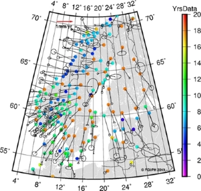
Figure 1. BIFROST GNSS velocities (vectors), their standard
uncertainties (ellipses) and length of time series (colored circles).
2.2 GIA velocities – NKG2016GIA_prel0907 model
The GIA model was computed using the software ICEAGE (Kaufmann, 2004)
which applies the viscoelastic normal-mode method (Peltier, 1974) and
where the sea-level equation is solved iteratively. A set of spherically
symmetric (1D), compressible, Maxwell-viscoelastic earth models with
four layers is generated. They differ in five parameters: lithospheric
and asthenospheric thickness, asthenospheric, upper and lower mantle
viscosity. Rheological parameters for the elastic structure are based on
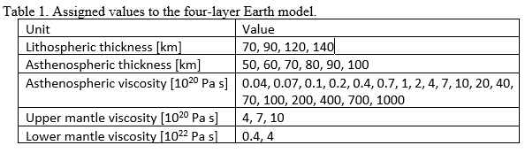
PREM (Dziewonski & Anderson, 1981). Table 1 summarizes the tested values
for the five parameters. Their range covers former results from the
computation of the land uplift model NKG2016LU (Vestøl et al.,
submitted).
Table 1. Assigned values to the four-layer Earth model.
We use a set of 25 different ice-sheet history model as surface
loads. These ice sheet chronologies for Fennoscandia, the Barents/Kara
seas and the British Isles are versions of GLAC (Tarasov et al. 2012,
Root et al. 2015, Nordman et al. 2015). Combination of these 25 ice
models with 2736 Earth models results in 68,400 unique GIA models to
test. For each GIA model, we calculate vertical elevation change (i.e.
the absolute land uplift), horizontal motion and sea-level change at
selected times during and after the last glaciation. This allows
comparison of our predictions with the BIFROST-derived GNSS result and a
large dataset of geological and paleontological relative sea-level (RSL)
observations for northern Europe (see Vestøl et al., submitted). The
observed velocity field is transformed into the GIA (model) frame
(Kierulf et al. 2014). We then compare and calculate the misfit of the
models to the observations with root-mean-square fitting:
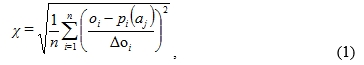
where, n is the number of observations considered, oi is the
observed RSL or BIFROST-derived velocity value, pi(aj) is the predicted
RSL or velocity for a specific GIA model aj, and Δoi is the data
uncertainty. The minimum value of χ within the parameter range
eventually results in the best-fitting Earth model ab. As we are
interested in a model that fits both the GNSS and RSL data
simultaneously, we calculate a linear weighted combination of the misfit
for GNSS data χGNSS and the misfit for RSL data χRSL to achieve a total
misfit χtotal. It is generally recommended to put more weight on the RSL
data to promote a unique solution (Vestøl et al., submitted). After some
tests, we give four times higher weight to RSL data than to the GNSS
data.
The best-fitting GIA model is called NKG2016GIA_prel0907. It consists
of a 120 km lithospheric thickness, a 90 km thick asthenosphere with a
viscosity of 1022 Pa s, an upper-mantle viscosity of 7 x 10²⁰ Pa s, a
lower mantle viscosity of 4 x 10²² Pa s and uses the GLAC ice history
model #71340. The horizontal velocity field of NKG2016GIA_prel0907 is
shown in Fig. 2.
3. METHODOLOGY
3.1 From a GIA frame to a geodetic reference frame
As the GIA velocities of the NKG2016GIA_prel0907 model are expressed
in a ”GIA frame” (Kierulf et al. 2014), they need to be re-aligned to a
geodetic reference frame. As mentioned in the previous section, GNSS
velocities can be used for reference frame alignment. As we want to
preserve the internal geometry of the GIA velocity model, we use a
Helmert fit with three rotations only to re-align the GIA velocities to
the GNSS velocities. This corresponds to an Euler pole approach and
affects only the horizontal velocities that we are interested in.
For alignment we select a subset of ”best” BIFROST stations
considering e.g. homogeneous distribution and length and discontinuities
of the GNSS time series. As a result 66 stations were used for alignment
of the GIA velocities (orange circles in Fig. 3). After the reference
frame alignment the GIA velocities agree with the GNSS velocities at
approx. 0.2-0.3 mm/a level (1σ), see Fig. 3. The uncertainty level of
the BIFROST velocities is, however, smaller and therefore we aim at
further improving the alignment. This is done with a least-squares
collocation.
3.2 Least-squares collocation (LSC)
After the Helmert fit, we use GNSS and aligned GIA velocities
together with GNSS velocity uncertainties as input to a least-squares
collocation, LSC. The LSC was performed with the GRAVSOFT software’s
routine GEOGRID component-wise, i.e. for North and East velocities
separately.
It is important to have as realistic standard uncertainties as
possible for the GNSS velocities in order to align the model well to the
GNSS velocities. By using power-law noise and estimating spectral index
for the uncertainty estimation, we consider the BIFROST velocity
uncertainties to be as realistic as possible. However, we still set the
minimum velocity uncertainty to 0.1mm/a in the LSC to avoid unncessary
instabilities in the collocation procedure.
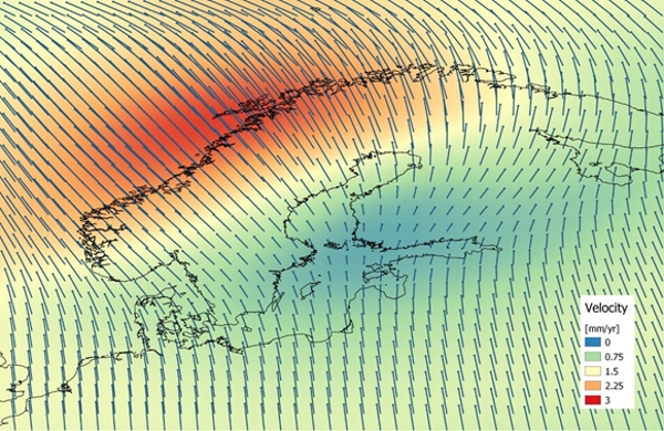
Figure 2. NKG2016GIA_prel0907 velocities.
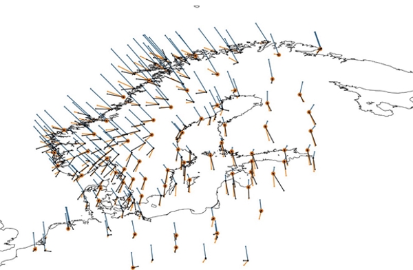
Figure 3. BIFROST (black vectors), NKG2016GIA_prel0907 (blue
vectors), re-aligned GIA (orange vectors) velocities and stations used
for alignment (orange circles).
GRAVSOFT models the covariance function with a second order
Gauss-Markov model where the user has to specify the correlation length.
Considering the density of CORS stations, expectation of a smooth
surface and the correlation length used in the NKG2016LU model, we
select the same 150 km correlation length for the horizontal velocities.
Farther away from CORS stations (basically outside the Nordic-Baltic
region) the model velocities converge to the aligned GIA velocities.
We use the ”remove-interpolate-restore” method meaning that we first
compute the velocity difference of the Helmert-fitted GIA velocities and
the GNSS velocities (remove GIA from the GNSS velocities), then apply
LSC to the velocity differences (collocation signal) and finally restore
the Helmert-fitted GIA velocities to the collocation signal to get the
intraplate model. The LSC also provides uncertainties for the obtained
signal. The collocation uncertainties are guided by the GNSS station
velocity uncertainties as well as the chosen correlation length. The
estimated signal, collocation uncertainty and the resulting intraplate
model are shown in Figs. 4, 5 and 6, respectively.
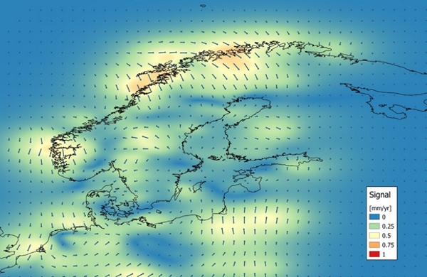
Figure 4. Least-squares collocation signal, i.e. correction on top of
the aligned GIA velocities.
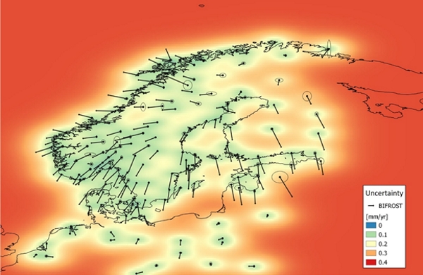
Figure 5. Least-squares collocation standard uncertainty.
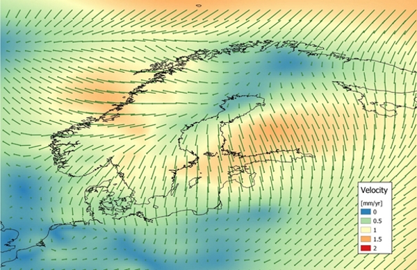
Figure 6. Velocities of the horizontal intraplate model.
4. RESULTS
4.1 Model minus BIFROST velocities
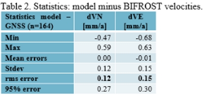
We compare the derived model and the BIFROST velocities in order to
verify the solution. Fig. 7 shows both velocities and BIFROST velocity
uncertainties. The model velocities converge to the BIFROST velocities
when the BIFROST velocity uncertainties are low and less with higher
uncertainties. The agreement, by means of root-mean-square (RMS) of
differences, has improved after the LSC from a 0.2-0.3 mm/a level to
0.12 mm/a and 0.15 mm/a for North and East velocities, respectively (see
Table 2). Consequently, the model agrees with the GNSS velocities at the
uncertainty level meaning optimum alignment with the available data.
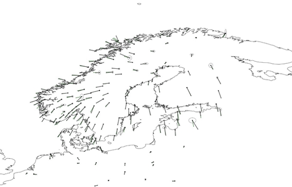
Figure 7. BIFROST (black vectors), model (green vectors) velocities
and BIFROST velocity uncer tainties (black ellipses).
Table 2. Statistics: model minus BIFROST velocities.
4.2 Model minus external GNSS velocities
Comparison in the previous section verifies the success of the
alignment of the model with respect to the used data. However, this
represents ”internal” accuracy of the model and it is therefore useful
to compare the model to some external data, too. We use a velocity
solution of the EPN (EUREF Permanent Network) densification project that
was released in 2018 (EPN 2019) for comparison. It covers whole Europe
with more than 3000 GNSS stations.
The EPN densification velocities are expressed in ETRF2000.
Therefore, we transformed our model to ETRF2000 before comparison. Then,
we interpolated the model velocities for the EPN densification stations.
There are almost 600 stations within the coverage of the model, however,
it must be noted that most of these are outside the Nordic-Baltic region
where the NKG model is guided rather by the GIA model than by GNSS
observations.
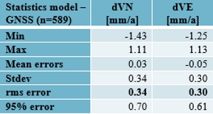
The agreement, by means of RMS of the differences, is at the level of
0.3 mm/a for the whole area of the model (Table 3). The agreement is,
however, better in the Nordic-Baltic area, see Fig. 8. This shows that
the model is working very well where the model is based on sufficiently
dense GNSS velocities. However, some less accurate regions can
immediately be seen from Fig. 8. It is obvious that the model suffers
from sparse GNSS data in the Baltic area as well as south to the Baltic
Sea e.g. in northern Germany and Poland. However, in this direct
comparison we did not consider any uncertainties which may explain part
of the differences. This is due to the fact that only unrealistic
white-noise type of uncertainties for the EPN densification velocities
are currently available.
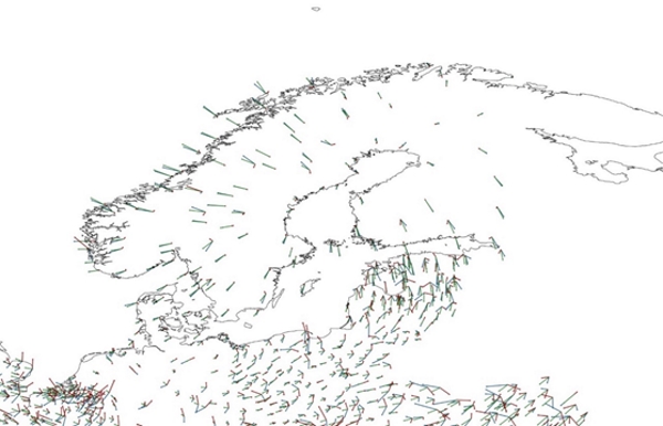
Figure 8. Model (green vectors), EPN densification (blue
vectors) velocities and their difference (red vectors).
Table 3. Statistics: model minus EPN densification velocities.
5. DISCUSSION
We have presented the methodology for development of a new horizontal
land uplift model for northern Europe. The model is based on GNSS and
GIA velocities and is a result of two consecutive alignments for the GIA
velocities. First, we do the reference frame alignment to get the GIA
velocities to a geodetic reference frame and then further align the
resulted velocities to agree with the GNSS velocities to a level of GNSS
uncertainties. We have shown this method to be successful but also
identified some small weaknesses in the current data set. The model is
lacking GNSS data in the Baltic region and south of the Baltic Sea and
in these areas the underlying GIA model is pronounced showing slightly
less accurate velocities. The model would benefit from extra data in
these areas. NKG is therefore preparing an updated GNSS velocity and
uncertainty solution for the Nordic-Baltic area that will include more
stations in the Baltic area as well as longer time series. This solution
will be released in the near future. Based on this and findings in this
paper, we will improve the model and therefore we consider this
model presented herein only as a preliminary model, NKG_RF17vel_prel.
We continue the work based on the findings in this paper.
A major finding is that the deformation pattern of the horizontal
velocities exhibits a source region, that is the area where velocities
are zero, further North than the location of the land uplift maximum
visible in NKG2016LU. Both locations are actually expected to overlap.
However, for NKG_RF17vel_prel intraplate velocities are reduced with the
ITRF2008-PMM from the IGb08 velocities. This model gives horizontal
velocities of a few tenths of mm/a to the area of vertical land uplift
maximum. The uncertainty of the absolute plate rotation pole of the
Eurasian plate from the ITRF2008-PMM is, by means of WRMS, about 0.3
mm/a for the fit stations (Altamimi et al. 2012). Considering this and
the fact that Fennoscandian GIA-affected stations were excluded from the
estimation of the Euler pole of the Eurasian plate, the agreement is at
the level that can be expected. One could improve this with an
additional fit by aligning the zero horizontal velocities to the
vertical land uplift maximum. On the other hand, considering usage of
the model, it is more likely that the model shall be used with the ITRF
plate motion model, cf. Häkli et al. 2016, and therefore it is not
meaningful to create a tailor-made solution. Besides, the situation may
be different when using other plate motion models. The updated NKG GNSS
solution will be expressed in ITRF2014, thus the corresponding
ITRF2014-PMM should consequently be used for reducing ITRF2014
velocities to intraplate velocities.
For this model we have used a correlation length of 150 km in the LSC
mainly based on the choice made for the vertical NKG2016LU model. We did
not perform a covariance analysis for the data but a test with a
correlation length of 200 km shows only negligible differences compared
to what was presented here. Influence on the model velocities was mainly
below 0.05 mm/a for the used BIFROST stations. But as we continue the
work, also a covariance analysis will be made before releasing the final
model.
In addition, we will produce uncertainties for the model velocities
and bring the model into a general use by incorporating it to the NKG
transformation scheme similarly as in Häkli et al. 2016.
REFERENCES
Altamimi, Z., Collilieux, X., Métivier, L. (2011): ITRF2008: an
improved solution of the international terrestrial reference frame. J.
Geod. 85, 457-473.
Altamimi Z., Métivier L. and Collieux X., 2012, ITRF2008 plate motion
model, J. Geophys. Res., 117, B07402. Doi:10.1029/2011JB008930.
Altamimi, Z., Rebischung, P., Métivier, L., Collilieux, X. (2016):
ITRF2014: A new release of the International Terrestrial Reference Frame
modeling nonlinear station motions. J. Geophys. Res. 121, 6109–6131.
Boehm, J., Werl, B., Schuh, H. (2006): Troposphere mapping functions
for GPS and very long baseline interferometry from European Centre for
Medium-Range Weather Forecasts operational analysis data. J. Geophys.
Res. 111, B02406.
Bos, M.S., Fernandes, R.M.S., Williams, S.D.P., Bastos, L. (2008):
Fast error analysis of continuous GPS observations. J. Geod. 82,
157–166, doi:10.1007/s00190-007-0165-x.
Dziewonski, A.M., Anderson, D.L. (1981): Preliminary reference Earth
model. Phys. Earth Planet. Inter. 25, 297–356.
EPN (2019): EPN densification:
http://epncb.oma.be/_densification/ Accessed February 1, 2019.
Herring T.A., King R.W., Floyd M.A., McClusky S.C. (2015):
Introduction to GAMIT/GLOBK Release 10.6. User Manual.
Häkli, P., Lidberg M., Jivall L., Nørbech T., Tangen O., Weber M.,
Pihlak P., Aleksejenko I., and Paršeliunas E., 2016, The NKG2008 GPS
campaign – final transformation results and a new common Nordic
reference frame, Journal of Geodetic Science. Volume 6, Issue 1, ISSN
(Online) 2081-9943, DOI: https://doi.org/10.1515/jogs-2016-0001, March
2016.
Kaufmann, G. (2004): Program package ICEAGE, Version 2004.
Manuscript, Institut für Geophysik der Universität Göttingen, 40 pp.
Kierulf, H.P. (2017): Analysis strategies for combining continuous
and episodic GNSS for studies of neo-tectonics in Northern-Norway. J.
Geodyn. 109, 32-40.
Kierulf, H.P., Steffen, H., Simpson, M.J.R., Lidberg, M., Wu, P.,
Wang, H. (2014): A GPS velocity field for Fennoscandia and a consistent
comparison to glacial isostatic adjustment models. J. Geophys. Res.
119(8), 6613-6629.
Lidberg M., Johansson J. M., Scherneck H.-G. and Milne G. A., 2010,
Recent results based on continuous GPS observations of the GIA process
in Fennoscandia from BIFROST, J. Geodyn, 50:1, 8–18.
Doi:10.1016/j.jog.2009.11.010.
Nordman, M., Milne, G., Tarasov, L. (2015): Reappraisal of the
Angerman River decay time estimate and its application to determine
uncertainty in Earth viscosity structure. Geophys. J. Int. 201,
811–822.
Nørbech T., Engsager K., Jivall L., Knudsen P., Koivula H., Lidberg
M., Madsen B., Ollikainen M. and Weber M., 2008, Transformation from a
Common Nordic Reference Frame to ETRS89 in Denmark, Finland, Norway, and
Sweden – status report, In: Knudsen P. (Ed.), Proceedings of the 15th
General Meeting of the Nordic Geodetic Commission (29 May – 2 June
2006), DTU Space, 68–75.
Peltier, W.R. (1974): The impulse response of a Maxwell earth. Rev.
Geophys. Space Phys. 12, 649-669.
Root, B.C., Tarasov, L., van der Wal, W. (2015): GRACE gravity
observations constrain Weichselian ice thickness in the Barents Sea.
Geophys. Res. Lett. 42, 3313–3320.
Scherneck, H.-G. (1991): A parametrized solid earth tide model and
ocean tide loading effects for global geodetic base-line measurements.
Geophys. J. Int. 106(3), 677-694.
Tarasov, L., Dyke, A.S., Neal, R.M., Peltier, W.R. (2012): A
data-calibrated distribution of deglacial chronologies for the North
American ice complex from glaciological modeling. Earth Planet. Sci.
Lett. 315–316, 30–40.
Vestøl O., 2006, Determination of postglacial land uplift in
Fennoscandia from leveling, tide-gauges and continuous GPS stations
using least squares collocation, J Geodesy, 80, 248–258. DOI
10.1007/s00190-006-0063-7.
Vestøl, O., Ågren, J., Steffen, H., Kierulf, H., Tarasov, L.
(submitted): NKG2016LU - A new land uplift model for Fennoscandia and
the Baltic Region. J. Geodesy.
Williams, S.D.P. (2008): CATS: GPS coordinate time series analysis
software. GPS Solutions 12, 147–153. doi:10.1007/s10291-007-0086-4.
Williams, S.D.P., Bock, Y., Fang, P., Jamason, P., Nikolaidis, R.M.,
Prawirodirdjo, L., Miller, M., Johnson, D.J. (2004): Error analysis of
continuous GPS position time series. J. Geophys. Res. 109, B03412,
doi:10.1029/2003JB002741.
Ågren J. and Svensson R., 2008, Land Uplift Model and System
Definition Used for the RH 2000 Adjustment of theBaltic Levelling Ring,
In: Knudsen P. (Ed.), Proceedings of the 15th General Meeting of the
Nordic Geodetic Commission (29 May – 2 June 2006), DTU Space, 84–92.
CONTACTS
Mr. Pasi Häkli
Finnish Geospatial Research Institute (FGI) / National Land Survey of
Finland Geodeetinrinne
2 Kirkkonummi
FINLAND
https://www.maanmittauslaitos.fi/en/research


