The Carmel Mountains Precise Geoid
by Dan Sharni & Haim B. Papo
Key words: Israel geoid, Stokes, gravity anomalies.
Abstract
This paper presents the final results of a
pilot-project, for mapping an accurate geoid of the State of Israel.
The purpose of the project was to develop a feasible methodology,
assemble all necessary data, design and test field procedures and
finally to work out a suitable analysis algorithm, including the
respective computer programs. The project was funded and supported by
the Survey of Israel over a period of five years between 1994 and
1999. An area of about 600-sq. km on and around the Carmel Mountains
served as a field laboratory and proving ground. The ultimate goal was
to render a geoid map of the pilot area with a one-sigma accuracy of 4
cm. The geoid map was compiled from three independent data sources
that complement each other:
-
Measured geoid undulations (indirectly -
by GPS and trigonometric leveling) at a network of control points.
The network density was set intentionally high by a factor of
three to four in order to provide means for testing the quality of
the map.
-
A global gravity model of the highest
order available. Over the years 1994-1999 a number of gravity
models were used, beginning with OSU'91, followed by EGM'96 and
finally - the 1800-order GPM'98B model.
-
A dense grid of free-air gravity anomalies
(3') extending up to a distance of 2o
from the pilot area. Within the state boundaries we used directly
measured anomalies. At sea and beyond the state boundaries we
depended on free-air gravity anomalies, reconstructed from a dense
Bouguer anomalies grid and a corresponding DTM of land-surface and
sea-floor topography.
The computational procedure based on the Remove
& Restore approach is as follows:
-
Transform the free-air-anomalies grid into a
grid of residual anomalies, by removing respective model (GPM'98B)
anomalies.
-
At every control point, compute model geoid
undulations (including a number of corrections such as "zero
order" undulation, the effect of global elevation, indirect
effect) and add Stokes integration of the residual free air
anomalies field.
-
Subtract from the above (b) "crude
prediction" the "measured" undulations and create a
control-point correction field. Interpolate the correction field
into a contour map or a grid. At any point within the grid
boundaries, geoid undulation can be predicted now by subtracting
the interpolated correction grid value from the "GPM'98B plus
Stokes" crude prediction.
Three factors dominate the accuracy of the final
geoid map:
-
Density of the anchor points.
-
Over-all fit of the gravity model to the local
geoid.
-
Radius of Stokes integration of the residual
free air anomalies field.
With anchor points spaced 5-20 km apart; employing
the GPM'98B model and finally extending Stokes integration up to 2o,
we obtained an accuracy (one-sigma) of 2 cm or better. Although our
accuracy estimates were based on sound analysis principles, they may
seem a bit too optimistic. Analysis of additional test fields should
confirm our "optimistic" results or else - define more
realistic accuracy estimates.
Dr. Dan Sharni
Geodesy
Technion
32000 Haifa
ISRAEL
Tel. + 972 4 829 2482
Fax + 972 4 823 4757
E-mail: sharni@techunix.technion.ac.il
Haim B. Papo
Geodesy
Technion
32000 Haifa
ISRAEL
Fax + 972 4 823 4757
E-mail: haimp@tx.technion.ac.il
The Carmel Mountains Precise Geoid
1. INTRODUCTION
The advent of "GPS leveling" and the need
for medium level accuracy and fast orthometric heights have renewed
the interest in precise geoid maps. In the past five years the authors
have been involved in a joint project with the Survey of Israel,
designed to develop and test surveying and analysis procedures for the
creation of a precise geoid for the State of Israel. The target
accuracy of geoid undulation differences between neighboring points
was set at 4 cm. An experimental laboratory was established in the
form of a pilot-project area on the Carmel Mountains near Haifa. A
dense network of some 70 control points was marked and surveyed in the
pilot-project area.
The project proceeded chronologically along two
distinct phases:
-
Field surveying and subsequent rigorous
adjustment of two complete and independent vertical control
networks (GPS and trigonometric leveling);
-
Collection of gravimetric and topographic data
of the pilot area and its neighborhood up to a radius of 2o
and development of optimal strategies and a respective algorithm
for modeling high-frequency variations of the geoid.
With the completion of phase (a) we had at our
disposal a network of 66 control points with an estimated accuracy of
undulation-differences between neighboring points of the order of 2
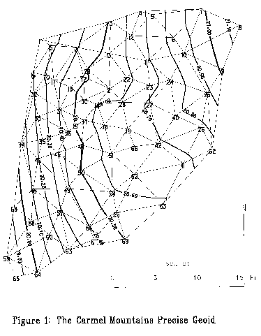
cm. Figure 1 shows a map of geoid undulations over the pilot-project
area based on all 66 points.
Phase (b) of the project was complicated and
lengthy, due to a severe lack of gravimetric data beyond the state's
boundaries. We applied data from various sources and modalities -
gravimmetry, DTM, bathymetry - to reconstruct and complement the
incomplete gravity-anomaly field. The well-known "Remove &
Restore" procedure, using a global gravity model, was then
utilized. We were able to bring our project to a successful conclusion
only after the introduction of a new gravity model (GPM'98B). GPM'98B
was the first global model to employ gravity data from our area.
2. MEASURED UNDULATION DIFFERENCES
Measured undulations (actually: computed
undulation-differences) were derived from GPS-height differences and
short-leg trigonometric leveling measured between points of a control
network. The total number of points with directly measured geoid
undulations was 66, where the pilot project covered an area of some
570 square km. The average distance between control points was thus
3-4 km, a rather dense spacing. The high density of control points was
intended to provide means for assessing undulation prediction quality
at different control point spacings.
GPS leveling
The observations were carried out by the Survey of
Israel, as a static GPS survey with 4 or 7 receivers. Each of the 66
control-points, as well as 10 more triangulation points (5 of which
were elevation benchmarks) was occupied for 2 sessions of 45 minutes
each /Sharni et.al, 1998/. Adjustment of the measured GPS vectors
resulted in a vertical control network with a standard deviation of
the order of 12 mm (8-15). The nominal accuracy might seem optimistic
but we found in the final analysis of the undulation-prediction
results that it was fairly representative.
Trigonometric Leveling
The pilot-project afforded the first opportunity,
in Israel, to analyze, write specifications, field-test and execute
extensive precise trigonometric leveling. The loop closures of the
measured elevation differences indicated that a 3rd-degree leveling
requirements (10.k1/2, where k is the loop-length in km)
can be readily met. Using 5" total-stations, limiting measuring
distances to a maximum of 120 m, pointing to the center of the
"coaxial" prism while it is supported on a tripod (not
hand-held) etc. were all part of a long list of specifications. In /Sharni
et.al., 1998/ we have reported in complete detail of our experiences
and achievements with trigonometric leveling. The final adjustment of
the measurements into a vertical control network (of orthometric
heights) produced a-posteriori error estimates that agreed very well
with our a-priori ones - indicating proper weighting of the
measurements. The estimated error per km came out 5.7 mm; the accuracy
of the adjusted elevation difference between points at 10-15 km
distance was 15 mm; the maximum error, propagated over the entire
project area (air-distance of the order of 40 km) reached only 22 mm.
Datum Considerations
The ellipsoidal (GPS) vertical network was adjusted
as a free network with datum derived from the nominal heights (WGS84)
of the above mentioned five benchmarks. We did not bother to
investigate how well the nominal heights of those benchmarks refer to
the WGS84 ellipsoid. We were reassured by their apparent consistency
(height differences) with our GPS measurements. The orthometric
vertical network was adjusted also as a free network. Here datum was
derived from the nominal heights of some 69 points as taken from the
catalogues of the first order vertical control network in Israel. Thus
the datum of our geoid undulations is as a matter of fact quite
arbitrary and is valid only within the limit of the pilot project. All
along in our pilot project we were interested in producing precise
undulation differences, which are datum-independent. Mapping the geoid
over the whole State of Israel is an entirely different story and
there appropriate measures will have to be taken to insure a uniform
datum. Estimated accuracies of our geoid undulations were derived from
the covariance matrices of the above two free vertical networks. To
generalize the results for the entire network we could say that
standard deviation of undulation-difference between any two
neighboring control-points 10-20 km apart is of the order of 20 mm. It
was comforting to know that we would have a wide margin of safety,
from our goal of prediction accuracy of 40 mm - even after
contributions to the error budget of representation and interpolation
would be accounted for.
3. MODELING GEOID VARIATIONS
In our project we counted on gravimmetry to provide
the means for modeling the finer details of the geoid surface. The
basic modeling tools were the well-known Remove & Restore process
and Stokes integration. The area in the proximity of the project is
covered by observed, discrete, gravity anomalies (and thus it can be
accounted for by Stokes integration). A global gravity model
represents the gravimmetry of the outlying areas (beyond the limits of
Stokes integration). Appropriate reductions and corrections are
applied to the data and model results, for compatibility.
Global gravity models
Initially we applied in our analyses the OSU'91A
model. We knew that this model did not incorporate enough data from
the Middle East, and consequently it may not be able to represent it
very well (it may not conform with our measured undulations). Later
on, NIMA released its EGM'96 model /Lemoine, 1998/, which contained
already some skeletal gravimmetric input from Israel. We received it
courtesy of Professor Richard H. Rapp, The Ohio State University. The
EGM'96 model seemed to fit better with our results - though we
encountered problems at sea, along the shore. Finally, Professor
Wenzel's model GPM'98B was put at our disposal after we did supply him
with gravity data from Israel. The 1800 order GPM'98B global gravity
model seemed to fit our measured undulations remarkably well.
Discrete gravity measurements
The Geophysical Institute (Dr. Yair Rotstein,
Director) made its file of observed gravity values available to our
project. It contained some 48,500 measured g values, mostly in Israel
and Sinai, between latitudes 27.7o-34.3
o and longitudes 32.4 o-36.1.
We applied atmospheric reductions and through the gravity-formula-1980
of /Moritz, 1980/ we produced "observed" free-air gravity
anomalies, on land. At a later date it was noticed (courtesy of the
late Professor Wenzel, then at The University of Karlsruhe, Germany),
that our observed gravity data had not been reduced to IGSN'71 - as
required to fit GF'80. The nominal reduction for Israel was of the
order of 12.5 mgal, whereas a cooperative effort between Israeli and
Jordanian scientists, investigating the Dead Sea area, suggested a
reduction of 15 mgal as more appropriate /Ten Brink, 1993/. This
reduction (15 mgal) was applied to the observed gravity data. The
point values were averaged into a regular, basic grid of 3 by 3
arc-minutes or 0.05 by 0.05 degrees (with a denser grid of 0.015 by
0.015 degrees within the project area).
The data included some obvious mistakes, as well as
blank areas, where not even one observation was available to compute
an average free-air anomaly for the respective cell. Those zeroes were
replaced by more realistic values, before applying Stokes integration.
We did this mostly by auto-correlation to neighboring cells.
Gravity data from other sources
Israel is a narrow state, with a mostly N/S extent.
On the west is the Mediterranean Sea. We did not have access to
gravity data from any of the neighboring states. The observed gravity
anomalies around the project area provided coverage of no more than
0.5 degrees in the north-east-south directions (land), while to the
west (sea) we had no data at all. The gravimmetric data was clearly
insufficient for a reliable Stokes integration. Thus it became
necessary to obtain indirect free-air anomalies, from other available
sources. An important source of gravity was a dense grid of Bouguer
anomalies of a wide area around the project, collected and collated by
the Geophysical Institute. From this we could reconstruct free-air
anomalies, utilizing available bathymetry of the East Mediterranean
(initially from Dr. John Hall, Geological Institute and later on from
US Naval Oceanographic Office). We needed also DTM data for free-air
anomaly reconstruction on land. We used at first Dr. Hall's DTM until
we obtained finally US Geological Survey (EROS) data - a dense grid of
30 by 30 arc-seconds). It was important to check the consistency
between bathymetry and DTM on land. In reconstructing free-air
anomalies over lakes, we took care of the unusual lake-surface
elevations in Israel (-210 m for Lake Kinneret and -405 m for Dead
Sea). In addition to water depths, we considered water-density (1.00
gr/cc for the Kinneret and 1.13 for the northern part of the Dead Sea;
maximum water density is close to 1.4! in the south). Some smoothing
was necessary, to fit reconstructed to observed anomalies, mainly
along the sea shore and the state borders. Thus we were able to
complete the construction of a grid of free-air anomalies extending
well beyond 2o from the borders of Israel. We regarded 2o
as a reasonable limit for Stokes integration.
The Remove & Restore Process
Following the well known R&R process we
employed the global gravity model GPM'98B to evaluate two free-air
anomalies grids corresponding exactly to our two grids of 0.05o
and 0.015o cell size. The grids of model anomalies were
subtracted (removed) from the respective average (or
reconstructed) grids thus producing two grids of residual anomalies.
The same model (GPM'98B) was used to evaluate height anomalies (a
first step towards the restoration of undulations) at each of
the 66 control points. We completed the computation of model geoid
undulations by applying a number of corrections to the height anomaly
and by adding the Stokes integral. The corrections were for
"zero-order" undulation, for the effect of global elevations
and for the indirect effect of the topography. At each control point
we added the result of Stokes integration of the residual free-air
anomalies field. The final result for each control point was regarded
as a "crude prediction" of its geoid undulation.
Stokes Integration
Two limits were defined for Stokes integration with
respect to any computation-point: the inner-limit related to the
specific grid cell within which the computation point is located, and
the outer-limit, beyond which integration is terminated. Stokes
integration between the computation-point and the inner-limit was
replaced by evaluation of the effect of a spherical cap. Several tests
were carried out to determine the optimal size of the inner-limit and
it was set finally at 0.44 of the finer grid size (0.015o).
The outer limit was set at 2o, as mentioned above. The
residual free air gravily anomalies for the project were arranged in a
basic grid of 0.05o, between latitudes 30.0o-35.5oand
longitudes 32.0o-38.0o. The finer grid 0.015o,
was reserved for the pilot area, between latitudes 32.4o-33.0o
and longitudes 34.7o-35.3o. Thus the total
result of Stokes integration at any point within the project area was
the sum of three integrals representing the spherical cap, the denser
grid and the basic grid.
Reductions from height-anomaly to geoid-undulation
The height-anomaly differs slightly from the geoid-undulation,
due to problems in the exact definition of the center-of-gravity of
the earth; the mass of the earth and the potential of the ellipsoid;
and height differences between the reference surfaces (telluroid,
elipsoid, geoid) and global topography. First, we apply the
"zero-order undulation" correction, estimated at -53 cm for
WGS'84 (subtract 53 cm from height-anomaly to obtain geoid-undulation).
Second, we compute the effect of the height differences. This
correction which was computed from EGM'96 harmonic coefficients came
out insignificantly small (a few mm only). The third (and last) was a
correction for the indirect-effect of topography potential, computed
by Grushinski's formula. It also came out rather moderate in size (in
the 0-2 cm range).
Undulation prediction algorithm
We summarize this section by listing the algorithm
for predicting geoid undulations within the borders of our pilot
project area. There are two distinct sequences:
Sequence a. Preparation of an undulation
correction grid (or contour map) based on a selected sub-network of
anchor points. Sequence (a) consists of the following steps:
-
a-1 at each anchor point evaluate the height
anomaly using a global gravity model.
-
a-2 at each anchor point perform Stokes
integration of residual f.a. anomalies.
-
a-3 for each anchor point evaluate corrections
for height anomalies / undulations.
-
a-4 sum a-1, a-2 and a-3 and subtract the directly
measured geoid undulation at the respective anchor points in order to create an
undulation correction field.
-
a-5 interpolate a-4 into a regular grid or a
contour map.
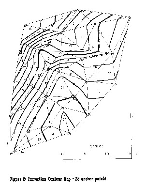
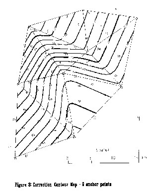
Figures 2 and 3 show two such correction contour
maps prepared for two different anchor point bases, where Stokes
integration (step a-2) was carried out up to an outer- limit of 2.0
degrees.
Sequence b. Prediction of geoid undulation at a
given position. Computational steps:
-
b-1 for the prediction point (f,l)
evaluate and sum a-1, a-2 and a-3.
-
b-2 interpolate a correction for (f,l)
using the a-5 grid (or contour map).
-
b-3 subtract b-2 from b-1 to obtain a prediction of
the geoid undulation at (f,l).
4. ANALYSIS OF EXPERIMENTS
Following the completion of the two leveling
campaigns and the subsequent analysis and adjustment of the
measurements we faced two problems regarding gravity data:
-
It was not clear how much the lack of
consistent and reliable gravity data beyond the state's boundaries
would affect the ultimate accuracy of undulation prediction. The
gravity anomalies field at our disposal allowed Stokes integration
only up to a distance (outer-limit) of 0.5o.
-
Up to 1997 the only gravity model at our
disposal was the OSU'91 model. The OSU model was developed without
the benefit of directly measured gravity data from our region. We
were not sure how much the above inherent deficiency of the model
is going to affect our R&R process and consequently - our
geoid undulation predictions.
Experiments with the new EGM'96 model in early 1998
brought a slight improvement to our predictions although we were still
confined to the 0.5o outer-limit for Stokes integration /Sharni
et.al., 1998/. In order to meet our target accuracy of 4 cm
(one-sigma) for an undulation difference within the project area we
still had to keep distances between the anchor points too short for
comfort (10 km in flat terrain and no more than 6 km in the mountain).
By mid 1998, equipped with the brand new GPM'98B gravity model, we
noted a much better fit to our directly measured undulations. Our
efforts to extend the limits of Stokes integration up to 2.0o
were at last (early 1999) crowned with success. We were finally ready
to perform a complete set of experiments and analyses.
We repeated Stokes integration (residual anomalies)
for a succession of outer-limits, beginning with 0.5oand up
to a maximum of 2.0o. The undulation correction field was
interpolated on the basis of 28 anchor points (distances of 8-12 km in
flat areas and 5-7 km in the mountain). Another set of interpolations
was based on only 9 anchor points, the distances being now 13-17 km
over the project area (see Figures 2 and 3).
Differences between predicted (b-3) and directly
measured undulations at the check points were used by us to estimate
the effective accuracy of the whole prediction process (See Table 1).
As check points we denoted all those control points which did not
serve as anchor points in preparing the undulation correction field
(a-4). Note that in spite of containing much less detail (See Figure
3), the 9 anchor points correction contour map produced predictions of
remarkably high accuracy. We went as far as to prepare a correction
field based on only 5 anchor points (not shown in this paper). The
resulting accuracy of prediction went down to 3 cm (one-sigma).
|
anchor points |
check points |
Stokes up to 0.5 o [mm] |
Stokes up to 2.0 o [mm] |
|
s |
max |
min |
>2s |
s |
max |
min |
>2s |
|
28 |
38 |
18 |
+52 |
-50 |
8% |
17 |
+45 |
-51 |
8% |
|
9 |
57 |
19 |
+52 |
-42 |
7% |
22 |
+55 |
-41 |
7% |
Table 1: Analysis of undulation prediction accuracy
(66 control points).
In Table 1 we summarize results of our analyses for
two outer-limits of integration. The remaining limits (0.8, 1.2 and
1.6 degrees) did not produce significantly different results so we
left them out. The pleasant surprise was that we were nicely below the
2 cm one-sigma level with our predictions. The above table brought
answers to both of our questions: (a) the best fitting properties of
the global gravity model are indeed crucial for deriving a precise
geoid in a given area; (b) the contribution of gravity anomalies
beyond 0.5o (50-60 km) can be defined at best as marginal.
|
point # |
1 |
2 |
3 |
4 |
5 |
6 |
7 |
8 |
9 |
10 |
11 |
|
difference |
234 |
253 |
241 |
237 |
246 |
256 |
250 |
247 |
253 |
256 |
261 |
|
point # |
12 |
13 |
14 |
15 |
16 |
17 |
19 |
21 |
22 |
23 |
24 |
|
difference |
251 |
252 |
261 |
239 |
241 |
255 |
260 |
266 |
259 |
263 |
262 |
|
point # |
25 |
26 |
27 |
28 |
29 |
30 |
31 |
32 |
33 |
34 |
35 |
|
difference |
258 |
258 |
265 |
265 |
259 |
263 |
266 |
251 |
257 |
275 |
268 |
|
point # |
36 |
37 |
38 |
39 |
40 |
41 |
42 |
44 |
45 |
46 |
48 |
|
difference |
276 |
271 |
271 |
267 |
264 |
261 |
262 |
281 |
282 |
280 |
289 |
|
point # |
49 |
50 |
51 |
52 |
53 |
54 |
55 |
56 |
57 |
58 |
59 |
|
difference |
295 |
287 |
279 |
286 |
270 |
288 |
290 |
287 |
296 |
288 |
295 |
|
point # |
60 |
61 |
62 |
63 |
64 |
65 |
66 |
68 |
69 |
70 |
72 |
|
difference |
293 |
292 |
255 |
299 |
293 |
291 |
267 |
289 |
287 |
242 |
258 |
Table 2: Contribution of Stokes integration between
0.5 and 2.0 degrees [mm].
The second conclusion (contrary to what we
expected) prompted an investigation of our intermediate results (not
shown in the paper) for an explanation. Table 2 shows a vector of
differences between a 0.5o "outer-limit" and a
2.0o "outer-limit" Stokes integration of residual
anomalies. Statistics of the vector, given in mm, are: average = 268;
variability = -34/+31; standard deviation = 17. Even more interesting
are the values for pairs of points at distances of 10-12 km. Compare,
for example, the differences at points 2, 23, 25, 33, 38, 42, 45, 54,
53, 56, 65 and 68 (See Table 2 and Figure 1). A simplistic
interpretation of the insignificant differences for neighboring points
is that the contribution of the residual gravity anomalies through
Stocks integration of cells between 0.5 and 2.0 degrees is practically
the same for points at distances of 10-12 km. We would like to confirm
the above conclusion in other parts of the country.
We have some reservations regarding the outcome of
our experiments. A prediction accuracy of the order of less than 20 mm
seems a bit "too good to be true". As stated above, error
analysis of the measured undulations following adjustment of the two
networks (GPS and trigonometric leveling) indicated accuracies of the
order of 2 cm for points at distances of 10-15 km. While the above
estimate seemed reasonable, it is hard to explain and to accept the
excellent prediction accuracies as shown in Table 1. There is no room
for the additional contributions to the error budget due to global
gravity model, Stokes integration, mode of interpolation etc. A number
of experiments in different parts of the country will have to be
carried out before we could claim that luck had nothing to do with our
results in the Carmel Mountain Pilot Project.
5. SUMMARY
We think that the primary objectives of our
pilot-project have been achieved. The success of modeling
high-frequency variations of geoid undulations by Stokes integration
of residual free air anomalies has been demonstrated. In order to
obtain undulation prediction accuracies as low as 2 cm, the distances
between directly measured undulations (at anchor-points) have to be
kept below the 15 km limit. However, if accuracies of 3-4 cm are
considered acceptable, then the above distances can be pushed beyond
the 20 km limit. Most of the data assembled and compiled for the
pilot-project, as well as relevant software packages that were
developed so far, were handed to the Survey of Israel and will be used
in its geoid mapping campaign.
References
1. H. Moritz, Geodetic Reference System
1980, BG, vol. 54 #3, 1980, pp. 395-405, 1980.
2. U.S. Ten Brink, et al, Structure of
the Dead Sea Pull-Apart Basin From Gravity Analysis, JGR, vol. 98
#B12, pp. 21,877-21,894, Dec. 1993.
3. F.G. Lemoine, et al, The Development
of the Joint NASA GSFC and the National Imagery and Mapping Agency
(NIMA) Geopotential Model EGM96, NASA, July 1998.
4. D. Sharni , H. Papo, Y. Forrai, The Geoid
In Israel: Haifa Pilot, Proceedings of the Second Continental Workshop
On The Geoid In Europe, Budapest, March 1998, edited by M. Vermeer and
J. Adams, Reports of the Finish Geodetic Institute, #98:4, pp.
263-270, 1998.
FIGURES
Dr. Dan Sharni
Geodesy
Technion
E-mail: sharni@techunix.technion.ac.il
Haim B. Papo
Geodesy
Technion
E-mail: haimp@tx.technion.ac.il
15 May 2000
|